The Sampling Demo
The Sampling Demo is a MATLAB GUI designed to show you the effects of
sampling continuous time signals. The Demo consists of two files:
sampling_demo.m and sampling_demo.fig.
To run the Demo, download both of these files to your home directory, change
to that directory in MATLAB, and type "sampling_demo"
at the command prompt.
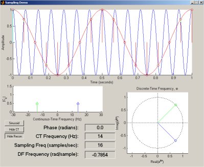
This demo has a number of features:
-
The edit boxes at the bottom of the figure allow you to set the continuous-time
frequency of a sinusoid (in Hz), it's phase (in radians), a sampling frequency
(in samples per second), and the discrete-time sampling frequency (in radians
per sample). Note that the DT frequency is determined by the CT frequency
and the sampling frequency.
-
Above these edit boxes is a display of the magnitude spectrum of the signal.
You can click-and-drag the spectral lines in this display to change the
frequency of the sinusoid. The blue line shows the "positive" frequency
component (which can be negative), and the green lines shows it's conjugate
pair.
-
The circular figure to the right of the edit boxes shows a schematic of
the circular nature of discrete time frequency. The lines shown indicate
location of the real and imaginary parts of ejw,
where w is the discrete-time frequency.
Note that w is given by the angle between the
point 1+j0 and the blue line. The green line shows its conjugate
pair. Note that you can also click-and-drag these lines around the
circle.
-
The top figure shows a continuous-time sinusoid (in blue) and the samples
of that continuous-time signal. Using the "Display CT/Hide CT" button,
you can turn on and off this blue curve. The "Display Recon/Hide
Recon" button also toggles a curve (in red) which shows the signal reconstructed
from the samples.
-
Finally, the button "Sinusoid/Complex Exponential" button converts the
signal under consideration from a sinusoid (which is composed of two complex
exponentials) to a single complex exponential. In "Complex Exponential"
mode, the top graph splits to show both real and imaginary parts of the
signal, while the spectral plot and DT frequency plots revert to only one
spectral line.
Some interesting things to notice:
-
Turn ON the reconstruction. Increase the frequency past fs/2.
What happens as the frequency passes fs/2?
-
Now increase it past fs. What happens as it passes fs?
-
Set the CT frequency equal to fs/2. What happens as you adjust the
phase of the sinusoid?